The CVM Algorithm

Everything you need to know about query planning can be understood from this query:

SELECT * FROM xy WHERE y = 3 ORDER BY x

Imagine we have two indexes, one ordered on y, and one ordered on x. Then two possible plans suggest themselves:

• Plan 1: scan the y index, restricting it to the values of y such that y = 3, then sort the result by x.
• Plan 2: scan the entire x index, selecting any rows having y = 3. The result will be "naturally" sorted by x, with no need for an extra sort.

We can come up with a cost model for each of these two approaches. Let |xy| be the size of the xy table and |q| be the number of rows in the result of the query. Then each plan costs:

Plan 1: |q| + |q|log|q|

Plan 2: |xy|

Which might look something like this:

It is the job of the query planner to choose between these two. In order to estimate the cost of each of these plans, we need to know |xy| and |q|. Or, at least, have a decent approximation of them. A common approach to this in databases is to periodically collect statistics about all of our relations. Maybe: every hour, scan all the tables and count the row in them. And maybe collect other information.

Let's assume for a second (and this is a bad assumption, but work with me), that xy is mostly uniformly distributed. That is, there are no like, super heavy values in it. Then, one way to approximate |q| is to know how many different values of y there are. If there are |Y| different values of |Y|, then we can approximate the number of rows with any particular value of y to be |xy|/|Y|.

This is just one example, but the point is that knowing |Y|, the number of distinct values for a particular column, is very useful.

Computing this is not particularly easy. If you want the exact answer, you need to do some kind of sorting, or build some kind of index structure to dedupe values. It turns out that if you just want an approximate value (like we do in query planning!), there are some alternative solutions.

The best and most popular algorithm for solving this problem is HyperLogLog. But there is a simpler, more fun algorithm for it that has come to be known as the CVM algorithm, originally introduced in the paper Distinct Elements in Streams: An Algorithm for the (Text) Book, made somewhat more widely known (and named) by Knuth's note on it.

I share Knuth's enthusiasm for the algorithm!

Their algorithm is not only interesting, it is extremely simple. Furthermore, it’s wonderfully suited to teaching students who are learning the basics of computer science. (Indeed, ever since I saw it, a few days ago, I’ve been unable to resist trying to explain the ideas to just about everybody I meet.) Therefore I’m pretty sure that something like this will eventually become a standard textbook topic.

So, let's state more precisely the problem being solved. We have a stream of elements, and we would like to know approximately how many different elements appear in that stream. Something like this:

def count_distinct(stream):
  seen = set()
  for v in stream:
    seen.add(v)
  return len(seen)

This implementation is certainly correct. We can test it against a sample input and see that it indeed always gives the correct results:

count_distinct(range(100000)) # -> 100000

I think a series of successive changes to this function are the best way to understand CVM. First, observe that this uses memory proportional to the number of distinct elements in the stream. We might try to cut down on the amount of memory we're using by only counting half the elements we see, and correct our result afterwards. We now say that each element has to win a coin flip to be included in the set:

def count_distinct(stream):
  seen = set()
  for v in stream:
    if random.random() < 0.5:
      seen.add(v)
  return len(seen) * 2

The idea is good, but this is wrong! Note that if we have a very long stream of all the same element, our result will reliably be 2, rather than a distribution centered at 1:

count_distinct([5,5,5,5,5]) # -> 2, most likely

We can plot the outputs to see if that is the case:

We want to make sure we only count every distinct element once. We can do this by blindly removing the element before we try inserting it again, in effect, only considering every element's final appearance to be the canonical one:

def count_distinct(stream):
  seen = set()
  for v in stream:
    seen.discard(v)
    if random.random() < 0.5:
      seen.add(v)
  return len(seen) * 2

Now our result is as we want: a distribution centered on the true value:

Every distinct value in stream is in seen with (independent) probability 0.5.

This cuts down the amount of memory we use by half. We can cut it down by an arbitrary amount by requiring more coin flips to be won for inclusion in the set (at the cost of variance):

flips = 3
def count_distinct(stream):
  seen = set()
  for v in stream:
    seen.discard(v)
    if random.random() < 1/2**flips:
      seen.add(v)
  return len(seen) * 2**flips

This is still only a constant amount of improvement, though. And more importantly, it doesn't let us bound the amount of memory used in total; there are inputs that will cause us to use arbitrarily high amounts of memory.

If flips is too large, we'll use too much memory. If flips is too small, the variance of our estimate will be high. What we want is to use a small value of flips for large datasets, and a large value of flips for small datasets. This gives us the final trick used in this algorithm, which is to pick the values of flips dynamically. We keep a bound on size, and if our set seen gets too large, we increment flips. We have to apply this standard to new elements along with the ones we've already seen. Since every element already in seen won flips flips, we can have them flip one more time to require them win flips+1 flips. Thus, the final algorithm is:

thresh = 1000 # how big our set is allowed to be
def count_distinct(stream):
  flips = 0
  seen = set()
  for v in stream:
    seen.discard(v)
    if random.random() < 1/2**flips:
      seen.add(v)
    while len(seen) == thresh:
      # require of each element in `seen` an additional flip
      seen = {v for v in seen if random.random() < 0.5}
      flips += 1
  return len(seen) * 2**flips

At the end of a run of this algorithm, every element is in the set with independent probability 1/2**flips. In other words, we have a bunch of identical and independently distributed random variables, which are very amenable to analysis.

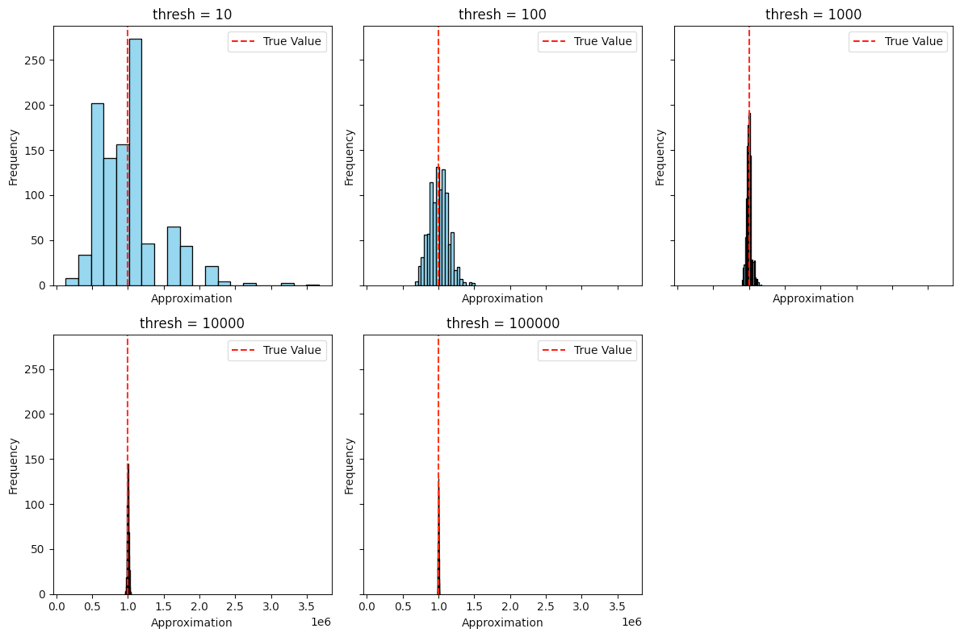
To confirm this algorithm actually works, we can plot a histogram of its outcomes. Note that to be "correct" here means that the distribution should be centered on the true value:

Note that as thresh gets larger, the variance of our estimate gets narrower and more reliably close to the true value, but no matter what, the distribution is always centered on the correct value: it's unbiased. Another perspective on this is to plot the mean of our run alongside the standard deviation:

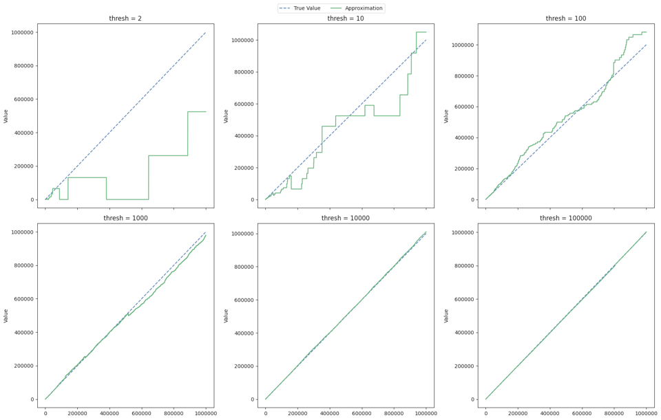
We can get a more intimate view of how one run of this algorithm behaves by plotting an individual run of it against the true size of a set. Here's what that looks like for various values of thresh:

If you actually need to solve this problem in production, you should probably just use HyperLogLog. It has a lot of nice properties, like being mergeable and having lots of high-quality implementations available. But this is my favourite algorithm because it's so simple to implement and easy to understand. If you're interested in doing theoretical analysis, HyperLogLog depends on subtle properties of the hash functions it uses for its correctness, whereas this does not depend on hashing for correctness at all.

Links

• Approximate Counting With Morris's Algorithm inspired some of the visualizations here (I found this via How Do Databases Count, another nice post).