September 22, 2025

I Misunderstood Rejection Sampling All This Time

If you’re like me, you have cobbled together an understanding of statistics following your mediocre second-year stats class by watching YouTube videos and skipping to sections of textbooks that are appropriate to the problem you are trying to solve at any particular moment and by asking your data scientists friends questions.

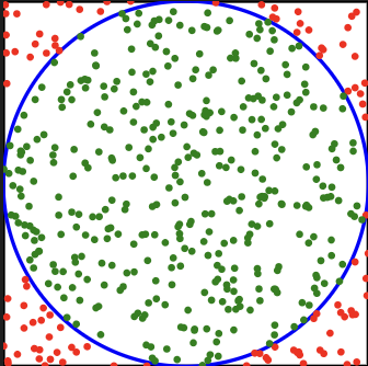
If you, like me, followed this route, you might know rejection sampling exclusively as “that thing people do to sample points on a disk.” To sample points on a disk:

• Sample points in the bounding box of the disk (this is easy because it’s two random() calls to sample in a rectangle),
• keep points that fall inside the disk.

If this is your exposure to rejection sampling, you might think that it can be characterized like so:

Take a uniform distribution (one that is easy to sample directly) whose sample space is a superset of some other uniform distribution’s sample space (one that is hard to sample directly) but for which you can test membership via some predicate. Sample points from the first sample space and only keep the ones that satisfy the predicate (in this case, that they’re less than 0.5 units in Euclidean distance from (1/2, 1/2)).

This is where, well, most YouTube videos stop, because the problem they’re trying to solve is usually sampling points on a disk. It turns out rejection sampling is a good bit more general than this!

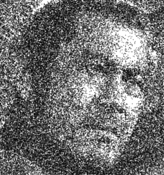
Imagine we want to sample points from an image like the following, at intensities proportional to the intensity of the pixels at a particular location:

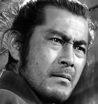
We can think of an image like this as a distribution, where the darker areas are more likely to be chosen than the lighter areas.

Let’s note a couple difficulties here:

• If the resolution of the image is very high, there might be too many pixels to reasonably treat this as a discrete distribution.
• We actually, a priori, don’t know the probability of a given pixel being chosen. Not without integrating across the entire image (which we could do) could we find the denominator we’d need to divide by to figure out the actual probability density function.

Nonetheless! We can sample this distribution in the following way:

• Pick a point uniformly on the image,
• generate a random number z in [0, 1),
• keep the point if its intensity is more than z.

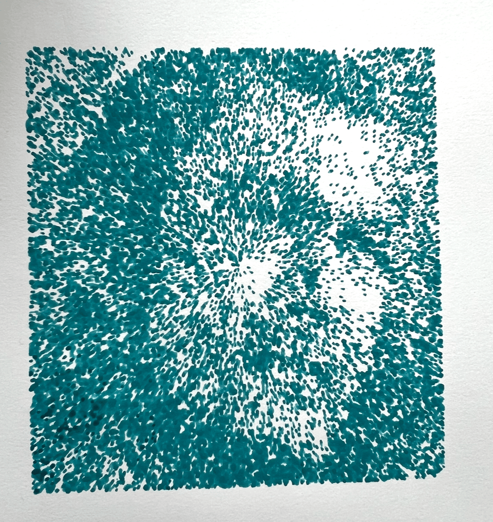
This works! It gives good results:

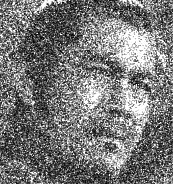
(100k attempted samples)

Okay, this secretly actually is the same as the “sampling a disk by sampling a square” trick: we’re sampling the unit-high rectangular prism that sits on top of the image, imagining each pixel sticks up with height proportional to its intensity, and then we check if our sample point sits within the image’s volume. This is really the same as doing the predicate thing we started with, but it feels more powerful, at least! We can extend this idea even further.

We are still actually not using the full power of rejection sampling. One observation you might make is we're being sort of wasteful: we're sampling across the whole image uniformly and then throwing away some of the points. In this example, we keep around 62% of the points. If we want to improve the efficiency, we could sample points more aggressively on the darker parts of the image. If we do this, we have to accommodate for that fact: if we make it harder to sample a lighter part of the image, it should be more likely we keep such a point than it otherwise would.

More generally, the rejection sampling algorithm is this:

Take two distributions F and G where:

• The density of F is at least as high as G everywhere,
• F is easy to sample,
• we can easily compute the density of G at a particular point.

Then, to sample from G:

• Sample r from F,
• keep r with probability G(r)/F(r) (where these are the "intensities," or some constant multiple of the probability density functions).

Our previous example is a special case where F is a uniform distribution.

So, what we can do, is split up the image into regions which we sample uniformly within:

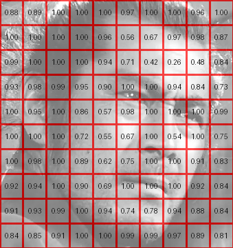
Then, we can mark each square with their max intensity, and sample them proportional to that max intensity using whatever method we please. You might think of this is subdividing up the image and then pushing down the roof of each subdivision until it touches the underlying image.

Once we pick a square, we can sample in there using the same rejection sampling as before. We get indistinguishable results:

But (slightly) better sampling efficiency (about 70%), that goes up if we make the boxes smaller, effectively shrink-wrapping our outer distribution atop our inner one.

If you've got a very steady hand, or maybe a robotic arm you can program, you can use this technique to do (sort of) renderings:

Anyway! This is just a reminder to actually look into algorithms you think you're familiar with in detail, a lot of the time you learn that there's a lot more to them than you realized.