We talked a couple issues ago about the application of Linearity of Expectation to building intuition about Copysets, and the ways that we're both constrained and freed by the laws of probability.

Evan recently pointed out a cool paper and writeup to me that can be understood in a similar way.

Here's the problem as he described it to me:

This is a really basic idea: generate unique IDs, in this case, that are going to be embedded in RocksDB SST files. The goal: don't have collisions, because maybe you want to move them around, put them in cloud object storage, etc.

Traditional approach: just pick a big random integer each time e.g. 128 bits.

Note that we're giving ourselves a couple restrictions here; processes don't necessarily get to "claim" a chunk of the ID-space by prefixing them with a name, or ID, or something. It's completely communication-free. Intuitively, it sort of smells as though this "pick random integer" approach should be optimal in some sense. But Evan followed up with:

The alternative: Each process starts by picking a random integer, but then just picks the next one.

The result: A much higher chance of having zero collisions.

This might be surprising to you, it was surprising to me! But the explanation makes sense for the same reasons that the Copysets explanation makes sense. You cannot change the expected number of collisions because expectation is linear. If I pick 100 IDs, out of a million, and you pick 100 IDs out of a million, we can compute the expectation like so. Let c_mn be 1 if my m-th ID collides with your n-th ID, and 0 otherwise. Then the number of collisions of a particular run is the sum of all of the cs:

Then the expectation of this is, by linearity:

In both strategies, any individual ID, ignoring all the others, is uniformly distributed across the entire space, so for all m and n, c_mn is constant, it's 1/1_000_000 since there's a million possible IDs to choose from.

So the expected number of collisions in either case is 1/100.

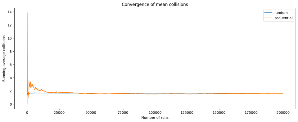
We can run a simulation to validate that the two strategies converge on the same mean number of collisions (but noting that the sequential approach takes longer to converge because of its higher variance):

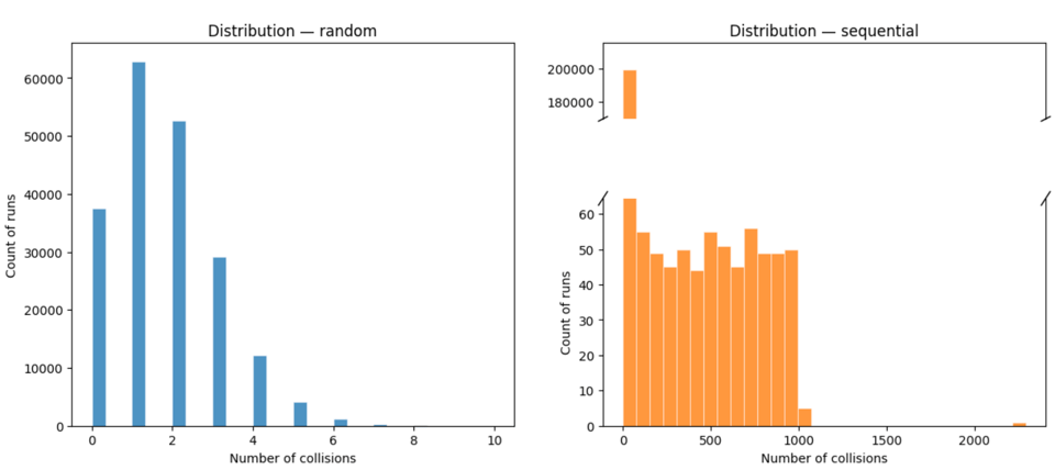
But the shape of the distributions is very different! The random strategy has a roughly Poisson distribution, with a big hump near the left side and a tail that hits zero quite fast, while the sequential strategy has a huge spike at "0 collisions" and a very long tail of high values:

We used this image last time to explain the difference between these kinds of situations:

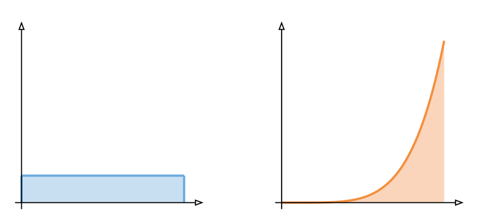
On the left, we have a uniform distribution, and on the right, a fat tailed distribution. Both have the same expectation: the area under the curve, but the two are shaped very differently and if you had a choice between them you might decide to pick one or the other.

I think this is another classic in the "fun and surprising applications of linearity of expectation" bucket! As an aside, this is my reminder for you that if you're a systems-y adjacent person a great way to have fun on computer is to learn to use Jupyter and enough Python to get by.