Edge Contractions and Join Planning

The join graph of a query has a vertex for each relation and an edge between any two relations that have a predicate between them.

For example, this query:

SELECT * FROM
  a, b, c, d, e, f, g
WHERE
      a.t = b.t
  AND b.u = c.u
  AND b.v = d.v
  AND d.w = e.w
  AND d.x = f.x
  AND d.y = g.y
  AND f.z = g.z

Has this join graph:

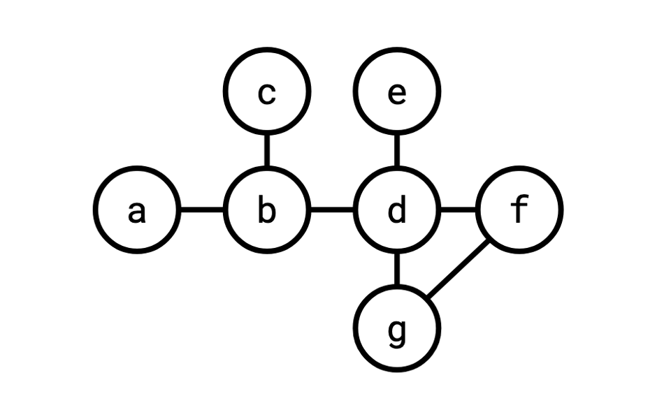
This is something of a heuristic object to be constructing in the general case. In SQL, you can use any kind of predicate for a join, so, you know, we could write WHERE b.q = e.q OR b.q != e.q and that would be a "predicate," but we're really interested in predicates that actually filter out some rows. And in reality, what we're mostly interested in is equality predicates, which are the most common kind of predicate (joins that use equality predicates are called equijoins, joins that use non-equality predicates are called theta joins).

Recall that the cross product of two relations is all the concatenations of rows from the two of them. It's what you get if you write

SELECT * FROM rel1, rel2

A "join" is a subset of the cross product. A cross product followed by a filtering of that cross product.

Actually ever computing a cross product is not desirable because it's very large. We'd rather compute something with a predicate on it so that we can use an algorithm like hash join or merge join .

Although most classical database systems can only join two tables at a time, the fact that joins are commutative (a join b = b join a) and associative (a join (b join c) = (a join b) join c) means this is sufficient to compute any join query: pick your two favourite tables, join them into a new one, and now we have a join query with one fewer table. We repeat until there's only one table left, and that's the result of the query.

This raises a question: what does this operation look like on the join graph? If we indeed pick our two favourite relations and join them, what's the effect on the join graph?

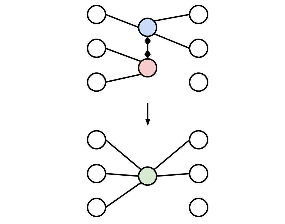
First of all, we merge the two vertices corresponding to the original table into one.

Next, when we join two relations, the resulting relation has the column set of both of the inputs. Thus, any predicates that were valid over either of the original tables are also valid over the resulting joined table. This means that any edges that were adjacent to the original two tables are now adjacent to the joined table, so we can re-connect any edges from the old vertices to the new one.

There's a simpler characterization of this operation though. In some sense, we're simply "forgetting" the distinction between the two input vertices, and pretending we are no longer able to distinguish them. This process is sometimes called identification: we're identifying two vertices by asserting they are "identical."

In the case where there was an edge between the original two vertices (which is the ideal case, remember, since we want to avoid computing cross products) this operation is known as edge contraction, where we squeeze an edge until its so short the two vertices become one:

The problem of join ordering is to decide what order to identify vertices in in order to compute the join with the least work. Lots of work has gone into understanding this.

One simple approach is to just avoid cross products. This is actually pretty easy, any kind of "traversal" of the graph will produce it. You can just pick a vertex and keep joining in adjacent vertices until you're done (of course, this doesn't work if the original graph is not connected, but it at least minimizes the number of cross products you will perform if you perform it for each component of the graph).

There's lots of ways to do this, you could pick two vertices and walk outwards from both of them in parallel, only joining the two components when they meet. Or, you could fix an order of the vertices ahead of time and maintain a set of disjoint components. There's a lot of ways to do it.

This technique of only allowing non-cross-product joins is important for algorithms that want to enumerate the entire join space as a way to restrict the size of it, for at least some join graph shapes, it's feasible to enumerate all the possible cross-product-free join orders without too much fuss.

Contracting edges repeatedly like this will eventually produce a join plan, or a binary tree that describes the order in which to join relations. This is the familiar thing you will often see if you run EXPLAIN on a SQL query, it's the tree through which tuples flow in the execution of a query.

To reconstruct the join plan from the sequence of edge contractions, whenever we perform an edge contraction, we combine the two relations we're merging with a join:

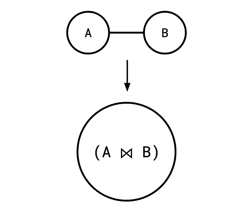
Repeating this process recursively, we eventually wind up with the final vertex containing an expression representing the join plan.

This is a very simplified approach to thinking about join ordering, it ignores things like statistics, indexes, outer joins, and different join algorithms, but it is an important intuitional foundation.