Remez Exchange Algorithm
Remember that the research plan for this essay series had four components
rational approximation
Remez' exchange algorithm
asymptotic series expansion
Taylor series expansion
I've deviated from the plan slightly by combining the last two bullet points into a single essay on the Maclaurin series, which is an asmptotic expansion and a generalization of Taylor. Using the key idea regarding the minimax approximation, we're ready to apply Remez' exchange algorithm.
We start with the minimax norm, and we write down a boundary on our total error like so

And the objective of our algorithm will be to find an approximation p(x) that has an error less than or equal to a parameter epsilon. Actually, for our purposes, we want the relative error at each specific value x, which is written

The reasons for using the relative error have to do with the behavior of the floating point representation, which we'll elide for now and revisit later.
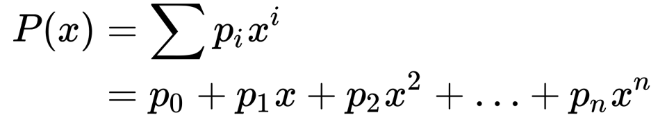
Evgeny Remez stated an iterative algorithm in 1934 that achieves our goal. First, we write down an approximation with the coefficients undefined
Next, substitute into the bounded error expression and observe that each attempt will be one of
equal to epsilon, in which case we've found an exact match and stop
less than epsilon
greater than epsilon
which we can write as a series of attempts. Here's the full derivation. Take the relative error

Multiply through by x and observe that each iteration will be either positive or negative with respect to the iteration k.

and rearrange to observe the right hand side will be a constant, and the left hand side contains our unknowns.

Finally, we iterate over these stages:
Choose a set of
k = n + 1values forx, with each value greater than the previous.solve k equations for the coefficients
preplace the reference set, and iterate from (2)
Chebyshev "Control Points"
The first stage will be satisfied by selecting what are known as Chebyshev control points. Given an interval [a, b], we'll find the midpoint and the split the semicircle above the midpoint into arcs of equal length. The equation for this is
and if we assume our interval is from zero to one, we have
Setting n = 10 gives the values
k | cos(kπ/10) | 0.5 + 0.5 cos(kπ/10) |
|---|---|---|
0 | 1 | 1 |
1 | 0.95106 | 0.97553 |
2 | 0.80902 | 0.90451 |
3 | 0.58799 | 0.79390 |
4 | 0.30902 | 0.61545 |
5 | 0 | 0.5 |
6 | -0.30902 | 0.34549 |
7 | -0.58799 | 0.20611 |
8 | -0.80902 | 0.09549 |
9 | -0.95106 | 0.02447 |
10 | -1 | 0 |
In the spirit of working from first principles, I computed the table by hand, using some known decimal values for the cosine function, and then verified my handiwork in a Jupyter Notebook.
System of Equations
The above table gives values to use for x_k. This will generate a system of equations with ten unknown coefficients. Solving these, using either Gauss-Jordan elimination or an LU decomposition, will give coefficent approximations.
Iterate
With the coefficent approximations created, we can then generate new, more accurate estimates on the interval. Doing this a few times will give us consistently better approximations. How? Look back at the convergence theorem in the previous essay!
That's a lot of work for now. Until next time!
You just read issue #7 of Software Archeology. You can also browse the full archives of this newsletter.