Minimax Approximation - Key Idea

If you've read my previous essay, you might have two questions: (1) how do you prove a Maclaurin series gives an accurate representation of its target function? (2) Why not use the generated series as a computational tool, rather than an approximation? The answer to the first question involves performing a repeated integration by parts on the target function. It's a fun exercise, but we'll leave that for another essay. Here, I want to briefly state why a series expansion falls short computationally, and how polynomial approximations rectify the situation.

Given a Maclaurin series for the error function

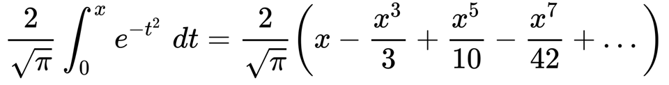
with only four terms written out, we have a polynomial that rapidly loses accuracy just before x = 1.

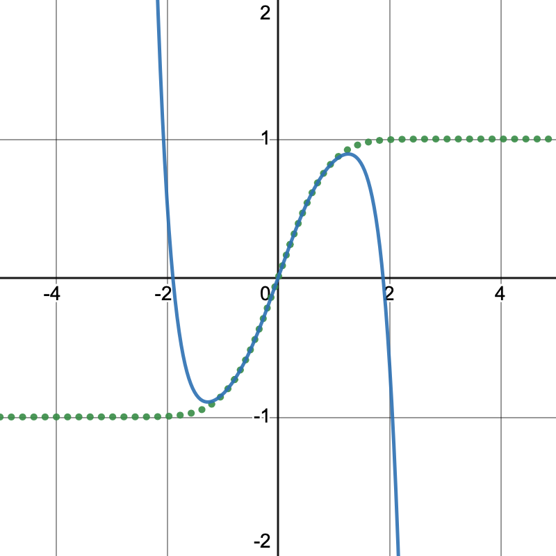
We could try to write out more terms, say to the sixth item in the series

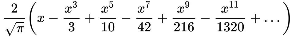
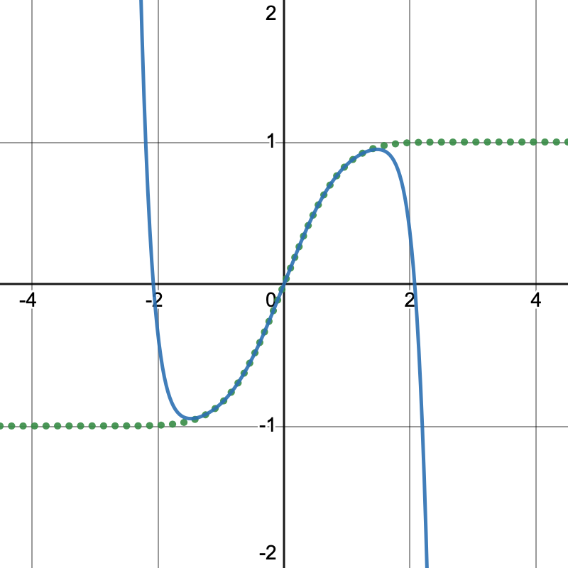
This persists a little past x = 1, but still rapidly loses accuracy prior to reaching x = 1.5. Thus we can see ourselves spending increasingly more computational energy for less accuracy gains.

That answers why we cannot use a series approximation outside a limited range: it's just too computationally expensive. The surprising -- and in some ways miraculous -- fact is that we can use a simpler, less expensive, i.e., more efficient, polynomial to obtain pretty good accuracy on a given range of inputs.

Let M_4 be an expansion to 4 terms and M_6 be an expansion to six terms. (note 1). For each point x, we can measure the difference in outputs from M_4(x) and M_6(x) like so

One of three things might happen when making this measurement:

• both series match exactly

• the series M_4 is greater than M_6

• the series M_6 is greater than M_4

We mostly need to know how far apart the series are, so we'll collapse the second two outcomes by taking the absolute value of the error

Now imagine we have a machine that computes the infinite Maclaurin series completely. We'll call this M_∞ This machine's impossible, but imagining it helps bound what's actually possible. We have

in particular, we want an approximation M_n that, as n approaches infinity, the absolute error approaches zero.This means we're looking to minimize the maximum error over all x

which is a mathematical structure known as an L_∞ norm.

So long as the function f is continuous on the interval of interest, an approximating polynomial P exists (note 2). Even better, we can invent a way to convert a function f to another continuous function in an ordered way. This sequence of functions will converge uniformly to the original function f (note 3).

The next task in our study will be to develop an "ordered way" to produce a function that converges to a desireable error bound.

Notes

• We could make the same demonstration using M_1 and M_2, but I've already given these two series as concrete examples. The logic works the same either way.

• The existance of a polynomial approximation is due to Weierstrauss; see Powell Theorem 6.1.

• For uniform convergence, see Powell Theorem 6.2

References

• M. J. D. Powell, Approximation Theory and Methods. Cambridge: Cambridge University Press, 1981. DOI